Extraction of Frequencies from Sinusoids with the Fast Fourier Transform in MATLAB

Vladimir Kulyukin

---

Problem
  

This post briefly describes how to plot and extract the frequency from single sinusoids in MATLAB with Fast Fourier Transform. Figure 1 shows a few important formulas that we will use.

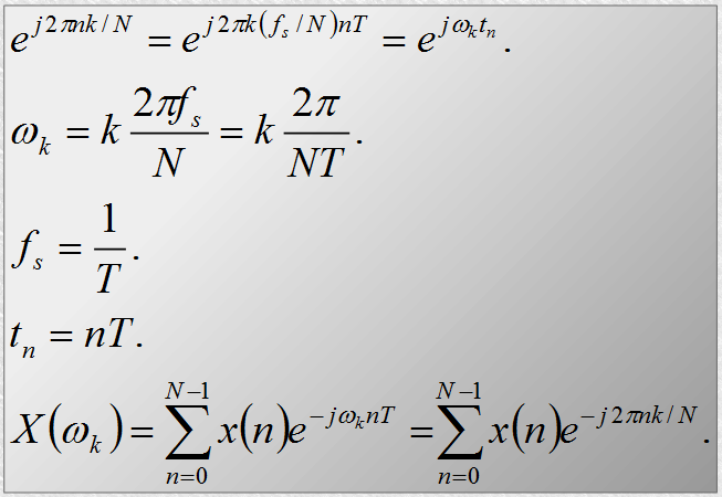Figure 1. FFT formulas

---

Defining Frequencies & Sinusoids

Let us define a few MATLAB constants. The k-constants below are used to define a few frequencies. We will set T and f_s  to 1, as is typically the case. A is an amplitude. We will not define N explicitly, i.e., number of time samples, because NT are common to all sinusoids and effectively acts as a scaling factor.

k1 = 50;
k2 = 120;
k3 = 150;
k4 = 170;
T = 1; %% time period
fs = 1/T;
A = 1;

Now we can define the frequencies and the time axis and sinusoids.

wk1 = k1*2*pi*fs;
wk2 = k2*2*pi*fs;
wk3 = k3*2*pi*fs;
wk4 = k4*2*pi*fs;

t = 0:0.001:0.6; %% from 0 upto 0.6 in increments of 0.0001. 
s = A*sin(wk1*t); %% sample sinusoid

---

Plotting the Time & Frequency Domains
 
We can start with defining the figure that has two subplots. The upper plot is the graph of a specific sinusoid, i.e., the signal in the time domain. The lower plot is the spectrum plot with the frequencies detected by the FFT.

figure(1);
subplot(3,1,1);

RightEndOfT = 100;  %% how far right to plot on the time axis
plot(1000*t(1:RightEndOfT),s(1:RightEndOfT), '-k'); grid off; %% plot the sinusoid without the grid

title('Sinusoid at k');
xlabel('Time (samples)');
ylabel('Amplitude');

Now we use the FFT to compute the spectrum and normalize it by the length of the time axis.

FFT_s = fft(s, length(t)); %% compute fft
NORM_FFT_s = FFT_s .* conj(FFT_s)/length(t); %% conjugate and normalize

All is left is to create the second subplot and label.

subplot(3, 1, 2);
RightEndOfNorm = 256; %% how far to plot to the right on NORM_FFT_s
ti = 1000*(0:RightEndOfNorm)/length(t);
plot(ti, NORM_FFT_s(1:RightEndOfNorm+1)); grid on;
xlabel('Frequency (cycles per sample)');
ylabel('Magnitude');

Figure 2 shows the results of plotting s = A*sin(wk1*t). Note that the frequency plot shows a spike at 50.

Figure 2. Time and frequency plots of s = A*sin(wk1*t) with a spike at wk1 = 50

Figure 3 shows the results of plotting s = A*sin(wk2*t). Note that the frequency plot shows a spike at 120.
 

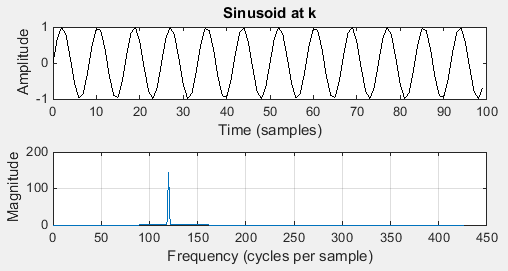Figure 3. Time and frequency plots of s = A*sin(wk2*t) with a spike at wk2=120

---

Extraction of Frequencies from Combined Sinusoids
 
We are now in the position to combine sinusoids and use the FFT to extract frequencies from these combined sinusoids. These examples are more realistic in that the real signals have multiple frequencies and noise. Figures 4 - 6 show the plots of different sinusoid combinations.
   

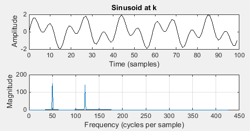Figure 4. Time and frequency plots of s = A*(sin(wk1*t)+sin(wk2*t)) with spikes at wk1=50, wk2=120

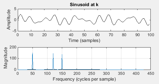Figure 5. Time and frequency plots of s =A*(sin(wk1*t)+sin(wk2*t)+sin(wk3*t)) with spikes at wk1=50, wk2=120, wk3=150

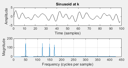Figure 6. Time and frequency plots of s = s = A*(sin(wk1*t)+sin(wk2*t)+sin(wk3*t)+sin(wk4*t)) with spikes at wk1=50,wk2=120, wk3=150, wk4=170.

---

MATLAB Source Code  

We can start with defining the figure that has two subplots. The upper plot is the graph of a specific sinusoid, i.e., the signal in the time domain. The lower plot is the spectrum plot with the frequencies detected by the FFT.

k1 = 50;
k2 = 120;
k3 = 150;
k4 = 170;
T = 1;
fs = 1/T;
A = 1;

wk1 = k1*2*pi*fs;
wk2 = k2*2*pi*fs;
wk3 = k3*2*pi*fs;
wk4 = k4*2*pi*fs;

t = 0:0.001:0.6; %% time axis in milliseconds
s = A*(sin(wk1*t)+sin(wk2*t)+sin(wk3*t)+sin(wk4*t));  %% sinusoid

RightEndOfT = 100;  %% how far to plot on the time axis
figure(1);
subplot(3,1,1);
plot(1000*t(1:RightEndOfT),s(1:RightEndOfT), '-k'); grid off;

title('Sinusoid at k');
xlabel('Time (samples)');
ylabel('Amplitude');

FFT_s = fft(s, length(t)); %% compute fft
NORM_FFT_s = FFT_s .* conj(FFT_s)/length(t); %% conjugate and normalize
subplot(3, 1, 2);
RightEndOfNorm = 256; %% how far to plot to the right on NORM_FFT_s
ti = 1000*(0:RightEndOfNorm)/length(t);
plot(ti, NORM_FFT_s(1:RightEndOfNorm+1)); grid on;
xlabel('Frequency (cycles per sample)');
ylabel('Magnitude');

---