
Problem
In this post, we will briefly discuss the relations between circles, sinusoids, amplitudes, radii, and phase offsets in FFT. Let the sinusoid be defined as A*sin(F*w+phi), where F is a positive integer and w is an angular frequency, e.g., 2*pi. Then there is a circle of radius A. The offset can be depicted on the circle as a segment that starts at the center of the circle (0, 0) and ends at (A*cos(phi), A*sin(phi)). On the sinusoid plot, the offset can be marked the amplitude axis (y-axis) at A*phi. The offset has no effect on the frequency spectrum plot.We will illustrate these relations in a series of simple and combined sinusoids. The complete source MATLAB source code is given at the end section of this post below.
Global Parameters
Let us define a few global parameters. Each global parameter is explained with a comment to the right of it. We will explain below why the SCALE variable is set 500 and how that value can be found.
phi = 0; %% phase offset; defaults to 0, try it with pi/2, pi/4, pi/10, etc.
t = 0:0.001:1; %% time x-axis
w = 2*pi; %% angular frequency
SCALE = 500; %% scale factor to make sure the spectrum plo is in [-A, +A], where A is as in
%% x = A*sin(F*w+phi).
ang=0:0.01:2*pi; %% angle array for drawing circles
sin01 = 1*sin(5*w*t+phi); %% sine curve 01; f = 5, amp = 1
We will do the FFT of the sinusoid, compute the absolute value of each entry, and divide each value by SCALE.
FFT_SIN_01 = abs(fft(sin01))/SCALE;
Now we can plot the sinusoid (Figure 1), the sinusoid's FFT spectrum (Figure 2), and the corresponding circle (Figure 3).
%% plot of sinusoid 01 shown in Figure 1.
figure(1);
plot(t, sin01);
xlabel('Time (s)')
ylabel('Amplitude')
title('1*sin(5*w*t)')
%% plot of sinusoid 01's spectrum shown in Figure 2.
figure(2);
plot(0:9, FFT_SIN_01(1:10));
xlabel('Frequency');
ylabel('Amplitude');
title('ABS(FFT(1*sin(5*w*t)))');
%% Plot of circle 01 the corresponds to sinusoid 01; plot is shown in Figure 03 below.
figure(3);
x1=0;
y1=0;
r1=1;
xp1=r1*cos(ang);
yp1=r1*sin(ang);
plot(x1+xp1,y1+yp1);
hold on;
plot([0,r1*cos(phi)], [0, r1*sin(phi)]);
title(strcat('Circle with r=1, phi=', num2str(phi)));
Note that in Figure 2 the frequency value at 5 is equal to 1, as is the case with 1*sin(5*w*t+phi). Why triangle instead of just a single line? My best guess is that this is due to the graphing interpolation that MATLAB does. If you display the contents of the FFT_SIN_01 array, the values of 500 are at indices 6 and 996 (1001-5=6), both of which correspond to the frequency of 5, due to the symmetry of the FFT spectra. The other values are all below 10, which can be verified as follows:
>> find(FFT_SIN_01>10)
ans =
6 997
Why was the SCALE variable set to 500? Let us recompute the FFT spectrum without dividing each value of 500. The new graph is shown in Figure 2X. Note that the value of 1 corresponds to 500 at the amplitude axis. Hence, the value of the SCALE variable.
Let us investigate how the change of phase affects the graphs in Figures 1, 2, and 3. All we need to do is to set the value of the global variable phi to pi/4 and re-run the program.
phi = pi/4; %% phase offset; defaults to 0, try it with pi/2, pi/4, pi/10, etc.
The new graphs are given in Figures 1a, 2a, and 3a. The modified sinusoid in Figure 1a starts at 1*pi/4 = 0.7854 on the amplitude axis. The graph of the scaled FFT spectrum in Figure 2a is unmodified, as expected. The graph of the corresponding circle in Figure 3a has an offset shown by the radius drawn from [0, 0] and [A*cos(pi/4), A*sin(pi/4)].
sin02 = 2*sin(4*w*t+phi); %% sine curve 02; f = 4, amp = 2
We will do the FFT of the second sinusoid, compute the absolute value of each entry, and divide each value by SCALE.
FFT_SIN_02 = abs(fft(sin02))/SCALE;
Now we can plot the second sinusoid (Figure 4), the second sinusoid's FFT spectrum (Figure 5), and the corresponding circle (Figure 6). As expected, the amplitude in Figure 4 goes from 2 to -2, the frequency value of 5 in Figure 5 has the corresponding value of 2, and the circle's radius in Figure 6 is 2, which corresponds to the amplitude of the second sinusoid.
%% plot of sinusoid 2*sin(4*w*t+phi) shown in Figure 4
figure(4);
plot(t, sin02);
xlabel('Time (s)')
ylabel('Amplitude')
title('2*sin(4*w*t)')
%% plot of sinusoid 02's spectrum shown in Figure 5
figure(5);
plot(0:9, FFT_SIN_02(1:10));
xlabel('Frequency');
ylabel('Amplitude');
title('ABS(FFT(2*sin(4*w*t)))');
%% circle 02, shown in Figure 6.
figure(6);
x2=0;
y2=0;
r2=2;
xp2=r2*cos(ang);
yp2=r2*sin(ang);
plot(x1+xp2,y2+yp2);
hold on;
plot([0,r2*cos(phi)], [0, r2*sin(phi)]);
title(strcat('Circle with r=2, phi=', num2str(phi)));
sin03 = 3*sin(3*w*t+phi); %% sin curve 03; f = 3, amp = 3
We do the FFT of the third sinusoid, compute the absolute value of each entry, and divide each value by SCALE.
FFT_SIN_03 = abs(fft(sin03))/SCALE;
Now we can plot the third sinusoid (Figure 7), the third sinusoid's FFT spectrum (Figure 8), and the corresponding circle (Figure 9). As expected, the amplitude in Figure 7 goes from 3 to -3, the frequency value of 3 in Figure 8 has the corresponding value of 3, and the circle's radius in Figure 9 is 3, which corresponds to the amplitude of the second sinusoid.
%% plot of sinusoid 3*sin(3*w*t) shown in Figure 7
figure(7);
plot(t, sin03);
xlabel('Time (s)')
ylabel('Amplitude')
title('3*sin(3*w*t)')
%% plot of the spectrum of 3*sin(3*w*t) shown in Figure 8
figure(8);
plot(0:9, FFT_SIN_03(1:10));
xlabel('Frequency');
ylabel('Amplitude');
title('ABS(FFT(3*sin(3*w*t)))');
%% circle 03 corresponding to 3*sin(3*w*t) shown in Figure 9.
x3=0;
y3=0;
r3=3;
xp3=r3*cos(ang);
yp3=r3*sin(ang);
plot(x3+xp3,y3+yp3);
hold on;
plot([0,r3*cos(phi)], [0, r3*sin(phi)]);
title(strcat('Circle with r=3, phi=', num2str(phi)));
The MATLAB code given below has seven more simple sinusoids.
%% two more sin curves
sin04 = 4*sin(2*w*t+phi); %% sin curve 04; f = 2, amp = 4
sin05 = 5*sin(1*w*t+phi); %% sin curve 05; f = 1, amp = 5
%% cosine curves
cos01 = 1*cos(5*w*t+phi); %% cos curve 01; f = 5, amp = 1
cos02 = 2*cos(4*w*t+phi); %% cos curve 02; f = 4, amp = 2
cos03 = 3*cos(3*w*t+phi); %% cos curve 03; f = 3, amp = 3
cos04 = 4*cos(2*w*t+phi); %% cos curve 04; f = 2, amp = 4
cos05 = 5*cos(1*w*t+phi); %% cos curve 05; f = 1, amp = 5
You can run the MATLAB code to look at the graphs. We will skip them for the sake of space and proceed to the graphs of complex sinusoids obtained by adding simple sinusoids.
Complex Sinusoid 06
sin06 = sin01 + sin02;
We do the FFT of the sixth sinusoid, compute the absolute value of each entry, and divide each value by SCALE.
FFT_SIN_06 = abs(fft(sin06))/SCALE;
In the plots of the sixth sinusoid, we will keep the MATLAB figure numbers. Thus, the sixth sinusoid is shown in Figure 26, the sixth sinusoid's FFT spectrum is in Figure 27, and the corresponding circles of the two component sinusoids are shown in Figure 28.
%% plot of sinusoid 06 = sin01 + sin02 shown in Figure 26.
figure(26);
plot(t, sin06);
xlabel('Time (s)')
ylabel('Amplitude')
title('1*sin(5*w*t)+2*sin(4*w*t+phi)')
%% plot of sinusoid 06's spectrum shown in Figure 27.
figure(27);
plot(0:9, FFT_SIN_06(1:10));
xlabel('Frequency');
ylabel('Amplitude');
title('ABS(FFT(1*sin(5*w*t)+2*sin(4*w*t+phi)))');
The plot shown in Figure 27 shows two component frequencies, 4 and 5, and their corresponding amplitudes are 2 and 1, respectively.
%% two circles corresponding to the two component sinusoids of the sixth sinusoid.
figure(28);
plot(x1+xp1,y1+yp1);
hold on;
plot(x2+xp2,y2+yp2);
plot([0,r1*cos(phi)], [0, r1*sin(phi)]);
plot([0,r2*cos(phi)], [0, r2*sin(phi)]);
title(strcat('Circle with r1=1,r2=2, phi=', num2str(phi)));
phi = 0; %% phase offset; defaults to 0, try it with pi/2, pi/4, pi/10, etc.
t = 0:0.001:1; %% time x-axis
w = 2*pi; %% angular frequency
SCALE = 500; %% scale factor to make sure the spectrum plo is in [-A, +A], where A is as in
%% x = A*sin(F*w+phi).
ang=0:0.01:2*pi; %% angle array for drawing circles
Sinusoid 01
The first sinusoid is A*sin(F*w+phi), where A = 1, F = 5, and phi = 0.
sin01 = 1*sin(5*w*t+phi); %% sine curve 01; f = 5, amp = 1
We will do the FFT of the sinusoid, compute the absolute value of each entry, and divide each value by SCALE.
FFT_SIN_01 = abs(fft(sin01))/SCALE;
Now we can plot the sinusoid (Figure 1), the sinusoid's FFT spectrum (Figure 2), and the corresponding circle (Figure 3).
%% plot of sinusoid 01 shown in Figure 1.
figure(1);
plot(t, sin01);
xlabel('Time (s)')
ylabel('Amplitude')
title('1*sin(5*w*t)')
 |
| Figure 1. Plot of 1*sin(5*w*t+phi), phi=0 |
figure(2);
plot(0:9, FFT_SIN_01(1:10));
xlabel('Frequency');
ylabel('Amplitude');
title('ABS(FFT(1*sin(5*w*t)))');
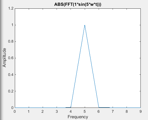 |
| Figure 2. Scaled FFT Spectrum of Sinusoid 01 |
figure(3);
x1=0;
y1=0;
r1=1;
xp1=r1*cos(ang);
yp1=r1*sin(ang);
plot(x1+xp1,y1+yp1);
hold on;
plot([0,r1*cos(phi)], [0, r1*sin(phi)]);
title(strcat('Circle with r=1, phi=', num2str(phi)));
Note that in Figure 2 the frequency value at 5 is equal to 1, as is the case with 1*sin(5*w*t+phi). Why triangle instead of just a single line? My best guess is that this is due to the graphing interpolation that MATLAB does. If you display the contents of the FFT_SIN_01 array, the values of 500 are at indices 6 and 996 (1001-5=6), both of which correspond to the frequency of 5, due to the symmetry of the FFT spectra. The other values are all below 10, which can be verified as follows:
>> find(FFT_SIN_01>10)
ans =
6 997
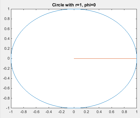 |
| Figure 3. Circle that Corresponds to 1*sin(5*w*t+phi), phi=0 |
Why was the SCALE variable set to 500? Let us recompute the FFT spectrum without dividing each value of 500. The new graph is shown in Figure 2X. Note that the value of 1 corresponds to 500 at the amplitude axis. Hence, the value of the SCALE variable.
 |
| Figure 2X. Unscaled Version of the FFT Spectrum Shown in Figure 2 |
phi = pi/4; %% phase offset; defaults to 0, try it with pi/2, pi/4, pi/10, etc.
The new graphs are given in Figures 1a, 2a, and 3a. The modified sinusoid in Figure 1a starts at 1*pi/4 = 0.7854 on the amplitude axis. The graph of the scaled FFT spectrum in Figure 2a is unmodified, as expected. The graph of the corresponding circle in Figure 3a has an offset shown by the radius drawn from [0, 0] and [A*cos(pi/4), A*sin(pi/4)].
 |
| Figure 1a. Plot of 1*sin(5*w*t+pi/4). |
 |
| Figure 2a. FFT Spectrum of 1*sin(5*w*t+pi/4) |
 |
| Figure 3a. Circle that Corresponds to 1*sin(5*w*t+pi/4) |
Sinusoid 02
The second sinusoid is A*sin(F*w+phi), where A=2, F=4, and phi=0.
sin02 = 2*sin(4*w*t+phi); %% sine curve 02; f = 4, amp = 2
We will do the FFT of the second sinusoid, compute the absolute value of each entry, and divide each value by SCALE.
FFT_SIN_02 = abs(fft(sin02))/SCALE;
Now we can plot the second sinusoid (Figure 4), the second sinusoid's FFT spectrum (Figure 5), and the corresponding circle (Figure 6). As expected, the amplitude in Figure 4 goes from 2 to -2, the frequency value of 5 in Figure 5 has the corresponding value of 2, and the circle's radius in Figure 6 is 2, which corresponds to the amplitude of the second sinusoid.
%% plot of sinusoid 2*sin(4*w*t+phi) shown in Figure 4
figure(4);
plot(t, sin02);
xlabel('Time (s)')
ylabel('Amplitude')
title('2*sin(4*w*t)')
 |
| Figure 4. Graph of 2*sin(4*w*t+phi), phi=0 |
figure(5);
plot(0:9, FFT_SIN_02(1:10));
xlabel('Frequency');
ylabel('Amplitude');
title('ABS(FFT(2*sin(4*w*t)))');
 |
| Figure 5. FFT Spectrum of 2*sin(4*w*t+phi), phi=0 |
figure(6);
x2=0;
y2=0;
r2=2;
xp2=r2*cos(ang);
yp2=r2*sin(ang);
plot(x1+xp2,y2+yp2);
hold on;
plot([0,r2*cos(phi)], [0, r2*sin(phi)]);
title(strcat('Circle with r=2, phi=', num2str(phi)));
 |
| Figure 6. Circle Corresponding to 2*sin(4*w*t+phi), phi = 0 |
Sinusoid 03
The third sinusoid is A*sin(F*w+phi), where A = 3, 3 = 4, and phi = 0.
sin03 = 3*sin(3*w*t+phi); %% sin curve 03; f = 3, amp = 3
We do the FFT of the third sinusoid, compute the absolute value of each entry, and divide each value by SCALE.
FFT_SIN_03 = abs(fft(sin03))/SCALE;
Now we can plot the third sinusoid (Figure 7), the third sinusoid's FFT spectrum (Figure 8), and the corresponding circle (Figure 9). As expected, the amplitude in Figure 7 goes from 3 to -3, the frequency value of 3 in Figure 8 has the corresponding value of 3, and the circle's radius in Figure 9 is 3, which corresponds to the amplitude of the second sinusoid.
%% plot of sinusoid 3*sin(3*w*t) shown in Figure 7
figure(7);
plot(t, sin03);
xlabel('Time (s)')
ylabel('Amplitude')
title('3*sin(3*w*t)')
 |
| Figure 7. Graph of 3*sin(3*w*t+phi), phi=0 |
figure(8);
plot(0:9, FFT_SIN_03(1:10));
xlabel('Frequency');
ylabel('Amplitude');
title('ABS(FFT(3*sin(3*w*t)))');
 |
| Figure 8. FFT Spectrum of 3*sin(3*w*t+phi), phi=0 |
x3=0;
y3=0;
r3=3;
xp3=r3*cos(ang);
yp3=r3*sin(ang);
plot(x3+xp3,y3+yp3);
hold on;
plot([0,r3*cos(phi)], [0, r3*sin(phi)]);
title(strcat('Circle with r=3, phi=', num2str(phi)));
 |
| Figure 9. Circle Corresponding to 3*sin(3*w*t+phi), phi=0 |
%% two more sin curves
sin04 = 4*sin(2*w*t+phi); %% sin curve 04; f = 2, amp = 4
sin05 = 5*sin(1*w*t+phi); %% sin curve 05; f = 1, amp = 5
%% cosine curves
cos01 = 1*cos(5*w*t+phi); %% cos curve 01; f = 5, amp = 1
cos02 = 2*cos(4*w*t+phi); %% cos curve 02; f = 4, amp = 2
cos03 = 3*cos(3*w*t+phi); %% cos curve 03; f = 3, amp = 3
cos04 = 4*cos(2*w*t+phi); %% cos curve 04; f = 2, amp = 4
cos05 = 5*cos(1*w*t+phi); %% cos curve 05; f = 1, amp = 5
You can run the MATLAB code to look at the graphs. We will skip them for the sake of space and proceed to the graphs of complex sinusoids obtained by adding simple sinusoids.
Complex Sinusoid 06
The sixth sinusoid is sin01 + sin02 = 1*sin(5*w*t+0) +2*sin(4*w*t+0) .
sin06 = sin01 + sin02;
We do the FFT of the sixth sinusoid, compute the absolute value of each entry, and divide each value by SCALE.
FFT_SIN_06 = abs(fft(sin06))/SCALE;
In the plots of the sixth sinusoid, we will keep the MATLAB figure numbers. Thus, the sixth sinusoid is shown in Figure 26, the sixth sinusoid's FFT spectrum is in Figure 27, and the corresponding circles of the two component sinusoids are shown in Figure 28.
%% plot of sinusoid 06 = sin01 + sin02 shown in Figure 26.
figure(26);
plot(t, sin06);
xlabel('Time (s)')
ylabel('Amplitude')
title('1*sin(5*w*t)+2*sin(4*w*t+phi)')
 |
| Figure 26. Graph of 1*sin(5*w*t)+2*sin(4*w*t), phi=0 |
figure(27);
plot(0:9, FFT_SIN_06(1:10));
xlabel('Frequency');
ylabel('Amplitude');
title('ABS(FFT(1*sin(5*w*t)+2*sin(4*w*t+phi)))');
 |
| Figure 27. FFT Spectrum of 1*sin(5*w*t)+2*sin(4*w*t+phi), phi=0 |
The plot shown in Figure 27 shows two component frequencies, 4 and 5, and their corresponding amplitudes are 2 and 1, respectively.
%% two circles corresponding to the two component sinusoids of the sixth sinusoid.
figure(28);
plot(x1+xp1,y1+yp1);
hold on;
plot(x2+xp2,y2+yp2);
plot([0,r1*cos(phi)], [0, r1*sin(phi)]);
plot([0,r2*cos(phi)], [0, r2*sin(phi)]);
title(strcat('Circle with r1=1,r2=2, phi=', num2str(phi)));
 |
| Figure 28. Two Circles Corresponding to the Two Component Sinusoids of Sinusoid 06 |
The seventh sinusoid is sin01 + sin02 + sin03 = 1*sin(5*w*t+0) +2*sin(4*w*t+0)+3*sin(3*w*t+0) .
sin07 = sin01 + sin02 + sin03;
We do the FFT of the seventh sinusoid, compute the absolute value of each entry, and divide each value by SCALE.
FFT_SIN_07 = abs(fft(sin07))/SCALE;
sin07 = sin01 + sin02 + sin03;
We do the FFT of the seventh sinusoid, compute the absolute value of each entry, and divide each value by SCALE.
FFT_SIN_07 = abs(fft(sin07))/SCALE;
We will again keep the MATLAB figure numbers. Thus, the seventh sinusoid is shown in Figure 29, the seventh sinusoid's FFT spectrum is in Figure 30, and the corresponding circles of the three component sinusoids are shown in Figure 31.
figure(29);
plot(t, sin07);
xlabel('Time (s)');
ylabel('Amplitude');
title('1*sin(5*w*t)+2*sin(4*w*t+phi)+3*sin(3*w*t+phi)');
 |
| Figure 29. Graph of 1*sin(5*w*t)+2*sin(4*w*t)+3*sin(3*w*t), phi=0 |
figure(30);
plot(0:9, FFT_SIN_07(1:10));
xlabel('Frequency');
ylabel('Amplitude');
title('ABS(FFT(1*sin(5*w*t)+2*sin(4*w*t+phi)+3*sin(3*w*t+phi)))');
 |
| Figure 30. FFT Spectrum of 1*sin(5*w*t)+2*sin(4*w*t)+3*sin(3*w*t), phi=0 |
figure(31);
plot(x1+xp1,y1+yp1);
hold on;
plot(x2+xp2,y2+yp2);
plot(x3+xp3,y3+yp3);
plot([0,r1*cos(phi)], [0, r1*sin(phi)]);
plot([0,r2*cos(phi)], [0, r2*sin(phi)]);
plot([0,r3*cos(phi)], [0, r3*sin(phi)]);
title(strcat('Circle with r1=1,r2=2,r3=3 phi=', num2str(phi)));
 | ||||||
| Figure 31. Graphs of the Circles Corresponding to the Sinusoids 1*sin(5*w*t)+2*sin(4*w*t)+3*sin(3*w*t), phi=0 |
Let us see what happens to the graphs of the seventh sinusoid when we set phi to pi/10. The graphs are given in Figures 29a, 30a, and 31a. As expected, the phase change is reflected in Figures 29a and 31a but has no effect on the FFT spectrum in Figure 30a.
 |
| Figure 29a. Graph of 1*sin(5*w*t+phi)+2*sin(4*w*t+phi)+3*sin(3*w*t+phi), phi=pi/10 |
 |
| Figure 30a. FFT Spectrum of 1*sin(5*w*t+phi)+2*sin(4*w*t+phi)+3*sin(3*w*t+phi), phi=pi/10 |
 |
| Figure 31a. Three Circles Corresponding to the Sinusoids 1*sin(5*w*t+phi)+2*sin(4*w*t+phi)+3*sin(3*w*t+phi), phi=pi/10 |
The 9th sinusoid combines both sine and cosine curves sin02+cos03+cos05 = 2*sin(4*w*t+phi)+3*cos(3*w*t+phi)+5*cos(1*w*t+phi), phi=0.
sin09 = sin02 + cos03 + cos05;
We do the FFT of the seventh sinusoid, compute the absolute value of each entry, and divide each value by SCALE.
FFT_SIN_09 = abs(fft(sin09))/SCALE;
The graphs of the sinusoid and the FFT spectrum are given in Figures 34 and 35. The circles are not plotted for the sake of space.
%% plot of sinusoid 09 = sin02 + cos03 + cos05
figure(34);
plot(t, sin09);
xlabel('Time (s)');
ylabel('Amplitude');
title('2*sin(4*w*t+phi)+3*cos(3*w*t+phi)+5*cos(1*w*t+phi)');
 |
| Figure 34. Graph of 2*sin(4*w*t+phi)+3*cos(3*w*t+phi)+5*cos(1*w*t+phi), phi=0 |
figure(35);
plot(0:9, FFT_SIN_09(1:10));
xlabel('Frequency');
ylabel('Amplitude');
title('ABS(FFT(2*sin(4*w*t+phi)+3*cos(3*w*t+phi)+5*cos(1*w*t+phi)))');
 |
| Figure 35. FFT Spectrum of 2*sin(4*w*t+phi)+3*cos(3*w*t+phi)+5*cos(1*w*t+phi), phi=0 |
%% ***********************************************************
%%
%% This program illustrates the relations between
%% circles, sinusoids, amplitudes, radii, and phase offsets
%%
%% Let the sinusoid be defined as x = A*sin(F*w+phi), where
%% F is a positive integer and w is an angular frequency, e.g.
%% 2*pi. Then there is a circle of radius A. The offset on the
%% circle can be depicted as a segment that starts at the
%% center of the circle (0, 0) and ends at (A*cos(phi), A*sin(phi)).
%% On the sinusoid plot, the offset is on the amplitude axis (y-axis)
%% A*phi. The offset has no effect on the frequency spectrum plot.
%%
%%
%% Author: Vladimir Kulyukin
%% ************************************************************
phi = 0; %% phase offset; defaults to 0, try it with pi/2, pi/4, pi/10, etc.
t = 0:0.001:1; %% time x-axis
w = 2*pi; %% angular frequency
SCALE = 500; %% scale factor to make sure the spectrum plot
%% is in [-A, +A], where A is as in
%% x = A*sin(F*w+phi).
ang=0:0.01:2*pi; %% angle array for drawing circles
%% sine curves
sin01 = 1*sin(5*w*t+phi); %% sin curve 01; f = 5, amp = 1
sin02 = 2*sin(4*w*t+phi); %% sin curve 02; f = 4, amp = 2
sin03 = 3*sin(3*w*t+phi); %% sin curve 03; f = 3, amp = 3
sin04 = 4*sin(2*w*t+phi); %% sin curve 04; f = 2, amp = 4
sin05 = 5*sin(1*w*t+phi); %% sin curve 05; f = 1, amp = 5
%% cosine curves
cos01 = 1*cos(5*w*t+phi); %% cos curve 01; f = 5, amp = 1
cos02 = 2*cos(4*w*t+phi); %% cos curve 02; f = 4, amp = 2
cos03 = 3*cos(3*w*t+phi); %% cos curve 03; f = 3, amp = 3
cos04 = 4*cos(2*w*t+phi); %% cos curve 04; f = 2, amp = 4
cos05 = 5*cos(1*w*t+phi); %% cos curve 05; f = 1, amp = 5
%% combined sinusoids
sin06 = sin01 + sin02;
sin07 = sin01 + sin02 + sin03;
sin08 = sin01 + cos01;
sin09 = sin02 + cos03 + cos05;
%%% FFT of all curves
FFT_SIN_01 = abs(fft(sin01))/SCALE;
FFT_SIN_02 = abs(fft(sin02))/SCALE;
FFT_SIN_03 = abs(fft(sin03))/SCALE;
FFT_SIN_04 = abs(fft(sin04))/SCALE;
FFT_SIN_05 = abs(fft(sin05))/SCALE;
FFT_SIN_06 = abs(fft(sin06))/SCALE;
FFT_SIN_07 = abs(fft(sin07))/SCALE;
FFT_SIN_08 = abs(fft(sin08))/SCALE;
FFT_SIN_09 = abs(fft(sin09))/SCALE;
%%% FFT of all curves
FFT_COS_01 = abs(fft(cos01))/SCALE;
FFT_COS_02 = abs(fft(cos02))/SCALE;
FFT_COS_03 = abs(fft(cos03))/SCALE;
FFT_COS_04 = abs(fft(cos04))/SCALE;
FFT_COS_05 = abs(fft(cos05))/SCALE;
%% ********* SINUSOID 01 PLOTS ***********
%% plot of sinusoid 01
figure(1);
plot(t, sin01);
xlabel('Time (s)')
ylabel('Amplitude')
title('1*sin(5*w*t)')
%% plot of sinusoid 01's spectrum
figure(2);
plot(0:9, FFT_SIN_01(1:10));
xlabel('Frequency');
ylabel('Amplitude');
title('ABS(FFT(1*sin(5*w*t)))');
%% circle 01
figure(3);
x1=0;
y1=0;
r1=1;
xp1=r1*cos(ang);
yp1=r1*sin(ang);
plot(x1+xp1,y1+yp1);
hold on;
plot([0,r1*cos(phi)], [0, r1*sin(phi)]);
title(strcat('Circle with r=1, phi=', num2str(phi)));
%% ********* SINUSOID 02 PLOTS ***********
%% 2*sin(4*w*t+phi)
%% plot of sinusoid 02
figure(4);
plot(t, sin02);
xlabel('Time (s)')
ylabel('Amplitude')
title('2*sin(4*w*t)')
%% plot of sinusoid 02's spectrum
figure(5);
plot(0:9, FFT_SIN_02(1:10));
xlabel('Frequency');
ylabel('Amplitude');
title('ABS(FFT(2*sin(4*w*t)))');
%% circle 02
figure(6);
x2=0;
y2=0;
r2=2;
xp2=r2*cos(ang);
yp2=r2*sin(ang);
plot(x1+xp2,y2+yp2);
hold on;
plot([0,r2*cos(phi)], [0, r2*sin(phi)]);
title(strcat('Circle with r=2, phi=', num2str(phi)));
%% ********* SINUSOID 03 PLOTS ***********
%% 3*sin(3*w*t)
%% plot of sinusoid 03
figure(7);
plot(t, sin03);
xlabel('Time (s)')
ylabel('Amplitude')
title('3*sin(3*w*t)')
%% plot of sinusoid 03's spectrum
figure(8);
plot(0:9, FFT_SIN_03(1:10));
xlabel('Frequency');
ylabel('Amplitude');
title('ABS(FFT(3*sin(3*w*t)))');
%% circle 03
figure(9);
x3=0;
y3=0;
r3=3;
xp3=r3*cos(ang);
yp3=r3*sin(ang);
plot(x3+xp3,y3+yp3);
hold on;
plot([0,r3*cos(phi)], [0, r3*sin(phi)]);
title(strcat('Circle with r=3, phi=', num2str(phi)));
%% ********* SINUSOID 04 PLOTS ***********
%% 4*sin(2*w*t)
%% plot of sinusoid 04
figure(10);
plot(t, sin04);
xlabel('Time (s)');
ylabel('Amplitude');
title('4*sin(2*w*t)');
%% plot of sinusoid 04's spectrum
figure(11);
plot(0:9, FFT_SIN_04(1:10));
xlabel('Frequency');
ylabel('Amplitude');
title('ABS(FFT( 4*sin(2*w*t)))');
%% circle 04
figure(12);
x4=0;
y4=0;
r4=4;
xp4=r4*cos(ang);
yp4=r4*sin(ang);
plot(x4+xp4,y4+yp4);
hold on;
plot([0,r4*cos(phi)], [0, r4*sin(phi)]);
title(strcat('Circle with r=4, phi=', num2str(phi)));
%% ********* SINUSOID 05 PLOTS ***********
%% sin05 = 5*sin(1*w*t)
figure(13);
plot(t, sin05);
xlabel('Time (s)');
ylabel('Amplitude');
title('5*sin(1*w*t)');
%% plot of sinusoid 05's spectrum
figure(14);
plot(0:9, FFT_SIN_05(1:10));
xlabel('Frequency');
ylabel('Amplitude');
title('ABS(FFT(5*sin(1*w*t)))');
%% circle 05
figure(15);
x5=0;
y5=0;
r5=5;
xp5=r5*cos(ang);
yp5=r5*sin(ang);
plot(x5+xp5,y5+yp5);
hold on;
plot([0,r5*cos(phi)], [0, r5*sin(phi)]);
title(strcat('Circle with r=5, phi=', num2str(phi)));
%% ************ COSINE CURVE FIGURES *****************
%% No circles are plotted.
%% cos01 = 1*cos(5*w*t)
figure(16);
plot(t, cos01);
xlabel('Time (s)');
ylabel('Amplitude');
title('1*cos(5*w*t)');
figure(17);
plot(0:9, FFT_COS_01(1:10));
xlabel('Frequency');
ylabel('Amplitude');
title('ABS(FFT(1*cos(5*w*t)))');
%% cos02 = 2*cos(4*w*t)
figure(18);
plot(t, cos02);
xlabel('Time (s)');
ylabel('Amplitude');
title('2*cos(4*w*t)');
figure(19);
plot(0:9, FFT_COS_02(1:10));
xlabel('Frequency');
ylabel('Amplitude');
title('ABS(FFT(2*cos(4*w*t)))');
%% cos03 = 3*cos(3*w*t)
figure(20);
plot(t, cos03);
xlabel('Time (s)');
ylabel('Amplitude');
title('3*cos(3*w*t)');
figure(21);
plot(0:9, FFT_COS_03(1:10));
xlabel('Frequency');
ylabel('Amplitude');
title('ABS(FFT(3*cos(3*w*t)))');
%% cos04 = 4*cos(2*w*t)figure(22);
plot(t, cos04);
xlabel('Time (s)');
ylabel('Amplitude');
title('4*cos(2*w*t))');
figure(23);
plot(0:9, FFT_COS_04(1:10));
xlabel('Frequency');
ylabel('Amplitude');
title('ABS(FFT(4*cos(2*w*t)))');
%% cos05 = 5*cos(1*w*t)
figure(24);
plot(t, cos05);
xlabel('Time (s)');
ylabel('Amplitude');
title('5*cos(1*w*t)');
figure(25);
plot(0:9, FFT_COS_05(1:10));
xlabel('Frequency');
ylabel('Amplitude');
title('ABS(FFT(5*cos(1*w*t)))');
%% ===== COMBINED SINUSOIDS
%% plot of sinusoid 06 = sin01 + sin02
figure(26);
plot(t, sin06);
xlabel('Time (s)')
ylabel('Amplitude')
title('1*sin(5*w*t)+2*sin(4*w*t+phi)')
%% plot of sinusoid 06's spectrum
figure(27);
plot(0:9, FFT_SIN_06(1:10));
xlabel('Frequency');
ylabel('Amplitude');
title('ABS(FFT(1*sin(5*w*t)+2*sin(4*w*t+phi)))');
%% two circles
figure(28);
plot(x1+xp1,y1+yp1);
hold on;
plot(x2+xp2,y2+yp2);
plot([0,r1*cos(phi)], [0, r1*sin(phi)]);
plot([0,r2*cos(phi)], [0, r2*sin(phi)]);
title(strcat('Circle with r1=1,r2=2, phi=', num2str(phi)));
%% plot of sinusoid 07 = sin01 + sin02 + sin03
figure(29);
plot(t, sin07);
xlabel('Time (s)');
ylabel('Amplitude');
title('1*sin(5*w*t)+2*sin(4*w*t+phi)+3*sin(3*w*t+phi)');
%% plot of sinusoid 07's spectrum
figure(30);
plot(0:9, FFT_SIN_07(1:10));
xlabel('Frequency');
ylabel('Amplitude');
title('ABS(FFT(1*sin(5*w*t)+2*sin(4*w*t+phi)+3*sin(3*w*t+phi)))');
%% circles corresponding to sin07
figure(31);
plot(x1+xp1,y1+yp1);
hold on;
plot(x2+xp2,y2+yp2);
plot(x3+xp3,y3+yp3);
plot([0,r1*cos(phi)], [0, r1*sin(phi)]);
plot([0,r2*cos(phi)], [0, r2*sin(phi)]);
plot([0,r3*cos(phi)], [0, r3*sin(phi)]);
title(strcat('Circle with r1=1,r2=2,r3=3 phi=', num2str(phi)));
%% plot of sinusoid 08 = sin01 + cos01
figure(32);
plot(t, sin08);
xlabel('Time (s)');
ylabel('Amplitude');
title('1*sin(5*w*t)+1*cos(5*w*t)');
%% plot of sinusoid 08's spectrum
figure(33);
plot(0:9, FFT_SIN_08(1:10));
xlabel('Frequency');
ylabel('Amplitude');
title('ABS(FFT(1*sin(5*w*t)+1*cos(5*w*t)))');
%% plot of sinusoid 09 = sin02 + cos03 + cos05
figure(34);
plot(t, sin09);
xlabel('Time (s)');
ylabel('Amplitude');
title('2*sin(4*w*t+phi)+3*cos(3*w*t+phi)+5*cos(1*w*t+phi)');
%% plot of sinusoid 09's spectrum
figure(35);
plot(0:9, FFT_SIN_09(1:10));
xlabel('Frequency');
ylabel('Amplitude');
title('ABS(FFT(2*sin(4*w*t+phi)+3*cos(3*w*t+phi)+5*cos(1*w*t+phi)))');
%%
%% This program illustrates the relations between
%% circles, sinusoids, amplitudes, radii, and phase offsets
%%
%% Let the sinusoid be defined as x = A*sin(F*w+phi), where
%% F is a positive integer and w is an angular frequency, e.g.
%% 2*pi. Then there is a circle of radius A. The offset on the
%% circle can be depicted as a segment that starts at the
%% center of the circle (0, 0) and ends at (A*cos(phi), A*sin(phi)).
%% On the sinusoid plot, the offset is on the amplitude axis (y-axis)
%% A*phi. The offset has no effect on the frequency spectrum plot.
%%
%%
%% Author: Vladimir Kulyukin
%% ************************************************************
phi = 0; %% phase offset; defaults to 0, try it with pi/2, pi/4, pi/10, etc.
t = 0:0.001:1; %% time x-axis
w = 2*pi; %% angular frequency
SCALE = 500; %% scale factor to make sure the spectrum plot
%% is in [-A, +A], where A is as in
%% x = A*sin(F*w+phi).
ang=0:0.01:2*pi; %% angle array for drawing circles
%% sine curves
sin01 = 1*sin(5*w*t+phi); %% sin curve 01; f = 5, amp = 1
sin02 = 2*sin(4*w*t+phi); %% sin curve 02; f = 4, amp = 2
sin03 = 3*sin(3*w*t+phi); %% sin curve 03; f = 3, amp = 3
sin04 = 4*sin(2*w*t+phi); %% sin curve 04; f = 2, amp = 4
sin05 = 5*sin(1*w*t+phi); %% sin curve 05; f = 1, amp = 5
%% cosine curves
cos01 = 1*cos(5*w*t+phi); %% cos curve 01; f = 5, amp = 1
cos02 = 2*cos(4*w*t+phi); %% cos curve 02; f = 4, amp = 2
cos03 = 3*cos(3*w*t+phi); %% cos curve 03; f = 3, amp = 3
cos04 = 4*cos(2*w*t+phi); %% cos curve 04; f = 2, amp = 4
cos05 = 5*cos(1*w*t+phi); %% cos curve 05; f = 1, amp = 5
%% combined sinusoids
sin06 = sin01 + sin02;
sin07 = sin01 + sin02 + sin03;
sin08 = sin01 + cos01;
sin09 = sin02 + cos03 + cos05;
%%% FFT of all curves
FFT_SIN_01 = abs(fft(sin01))/SCALE;
FFT_SIN_02 = abs(fft(sin02))/SCALE;
FFT_SIN_03 = abs(fft(sin03))/SCALE;
FFT_SIN_04 = abs(fft(sin04))/SCALE;
FFT_SIN_05 = abs(fft(sin05))/SCALE;
FFT_SIN_06 = abs(fft(sin06))/SCALE;
FFT_SIN_07 = abs(fft(sin07))/SCALE;
FFT_SIN_08 = abs(fft(sin08))/SCALE;
FFT_SIN_09 = abs(fft(sin09))/SCALE;
%%% FFT of all curves
FFT_COS_01 = abs(fft(cos01))/SCALE;
FFT_COS_02 = abs(fft(cos02))/SCALE;
FFT_COS_03 = abs(fft(cos03))/SCALE;
FFT_COS_04 = abs(fft(cos04))/SCALE;
FFT_COS_05 = abs(fft(cos05))/SCALE;
%% ********* SINUSOID 01 PLOTS ***********
%% plot of sinusoid 01
figure(1);
plot(t, sin01);
xlabel('Time (s)')
ylabel('Amplitude')
title('1*sin(5*w*t)')
%% plot of sinusoid 01's spectrum
figure(2);
plot(0:9, FFT_SIN_01(1:10));
xlabel('Frequency');
ylabel('Amplitude');
title('ABS(FFT(1*sin(5*w*t)))');
%% circle 01
figure(3);
x1=0;
y1=0;
r1=1;
xp1=r1*cos(ang);
yp1=r1*sin(ang);
plot(x1+xp1,y1+yp1);
hold on;
plot([0,r1*cos(phi)], [0, r1*sin(phi)]);
title(strcat('Circle with r=1, phi=', num2str(phi)));
%% ********* SINUSOID 02 PLOTS ***********
%% 2*sin(4*w*t+phi)
%% plot of sinusoid 02
figure(4);
plot(t, sin02);
xlabel('Time (s)')
ylabel('Amplitude')
title('2*sin(4*w*t)')
%% plot of sinusoid 02's spectrum
figure(5);
plot(0:9, FFT_SIN_02(1:10));
xlabel('Frequency');
ylabel('Amplitude');
title('ABS(FFT(2*sin(4*w*t)))');
%% circle 02
figure(6);
x2=0;
y2=0;
r2=2;
xp2=r2*cos(ang);
yp2=r2*sin(ang);
plot(x1+xp2,y2+yp2);
hold on;
plot([0,r2*cos(phi)], [0, r2*sin(phi)]);
title(strcat('Circle with r=2, phi=', num2str(phi)));
%% ********* SINUSOID 03 PLOTS ***********
%% 3*sin(3*w*t)
%% plot of sinusoid 03
figure(7);
plot(t, sin03);
xlabel('Time (s)')
ylabel('Amplitude')
title('3*sin(3*w*t)')
%% plot of sinusoid 03's spectrum
figure(8);
plot(0:9, FFT_SIN_03(1:10));
xlabel('Frequency');
ylabel('Amplitude');
title('ABS(FFT(3*sin(3*w*t)))');
%% circle 03
figure(9);
x3=0;
y3=0;
r3=3;
xp3=r3*cos(ang);
yp3=r3*sin(ang);
plot(x3+xp3,y3+yp3);
hold on;
plot([0,r3*cos(phi)], [0, r3*sin(phi)]);
title(strcat('Circle with r=3, phi=', num2str(phi)));
%% ********* SINUSOID 04 PLOTS ***********
%% 4*sin(2*w*t)
%% plot of sinusoid 04
figure(10);
plot(t, sin04);
xlabel('Time (s)');
ylabel('Amplitude');
title('4*sin(2*w*t)');
%% plot of sinusoid 04's spectrum
figure(11);
plot(0:9, FFT_SIN_04(1:10));
xlabel('Frequency');
ylabel('Amplitude');
title('ABS(FFT( 4*sin(2*w*t)))');
%% circle 04
figure(12);
x4=0;
y4=0;
r4=4;
xp4=r4*cos(ang);
yp4=r4*sin(ang);
plot(x4+xp4,y4+yp4);
hold on;
plot([0,r4*cos(phi)], [0, r4*sin(phi)]);
title(strcat('Circle with r=4, phi=', num2str(phi)));
%% ********* SINUSOID 05 PLOTS ***********
%% sin05 = 5*sin(1*w*t)
figure(13);
plot(t, sin05);
xlabel('Time (s)');
ylabel('Amplitude');
title('5*sin(1*w*t)');
%% plot of sinusoid 05's spectrum
figure(14);
plot(0:9, FFT_SIN_05(1:10));
xlabel('Frequency');
ylabel('Amplitude');
title('ABS(FFT(5*sin(1*w*t)))');
%% circle 05
figure(15);
x5=0;
y5=0;
r5=5;
xp5=r5*cos(ang);
yp5=r5*sin(ang);
plot(x5+xp5,y5+yp5);
hold on;
plot([0,r5*cos(phi)], [0, r5*sin(phi)]);
title(strcat('Circle with r=5, phi=', num2str(phi)));
%% ************ COSINE CURVE FIGURES *****************
%% No circles are plotted.
%% cos01 = 1*cos(5*w*t)
figure(16);
plot(t, cos01);
xlabel('Time (s)');
ylabel('Amplitude');
title('1*cos(5*w*t)');
figure(17);
plot(0:9, FFT_COS_01(1:10));
xlabel('Frequency');
ylabel('Amplitude');
title('ABS(FFT(1*cos(5*w*t)))');
%% cos02 = 2*cos(4*w*t)
figure(18);
plot(t, cos02);
xlabel('Time (s)');
ylabel('Amplitude');
title('2*cos(4*w*t)');
figure(19);
plot(0:9, FFT_COS_02(1:10));
xlabel('Frequency');
ylabel('Amplitude');
title('ABS(FFT(2*cos(4*w*t)))');
%% cos03 = 3*cos(3*w*t)
figure(20);
plot(t, cos03);
xlabel('Time (s)');
ylabel('Amplitude');
title('3*cos(3*w*t)');
figure(21);
plot(0:9, FFT_COS_03(1:10));
xlabel('Frequency');
ylabel('Amplitude');
title('ABS(FFT(3*cos(3*w*t)))');
%% cos04 = 4*cos(2*w*t)figure(22);
plot(t, cos04);
xlabel('Time (s)');
ylabel('Amplitude');
title('4*cos(2*w*t))');
figure(23);
plot(0:9, FFT_COS_04(1:10));
xlabel('Frequency');
ylabel('Amplitude');
title('ABS(FFT(4*cos(2*w*t)))');
%% cos05 = 5*cos(1*w*t)
figure(24);
plot(t, cos05);
xlabel('Time (s)');
ylabel('Amplitude');
title('5*cos(1*w*t)');
figure(25);
plot(0:9, FFT_COS_05(1:10));
xlabel('Frequency');
ylabel('Amplitude');
title('ABS(FFT(5*cos(1*w*t)))');
%% ===== COMBINED SINUSOIDS
%% plot of sinusoid 06 = sin01 + sin02
figure(26);
plot(t, sin06);
xlabel('Time (s)')
ylabel('Amplitude')
title('1*sin(5*w*t)+2*sin(4*w*t+phi)')
%% plot of sinusoid 06's spectrum
figure(27);
plot(0:9, FFT_SIN_06(1:10));
xlabel('Frequency');
ylabel('Amplitude');
title('ABS(FFT(1*sin(5*w*t)+2*sin(4*w*t+phi)))');
%% two circles
figure(28);
plot(x1+xp1,y1+yp1);
hold on;
plot(x2+xp2,y2+yp2);
plot([0,r1*cos(phi)], [0, r1*sin(phi)]);
plot([0,r2*cos(phi)], [0, r2*sin(phi)]);
title(strcat('Circle with r1=1,r2=2, phi=', num2str(phi)));
%% plot of sinusoid 07 = sin01 + sin02 + sin03
figure(29);
plot(t, sin07);
xlabel('Time (s)');
ylabel('Amplitude');
title('1*sin(5*w*t)+2*sin(4*w*t+phi)+3*sin(3*w*t+phi)');
%% plot of sinusoid 07's spectrum
figure(30);
plot(0:9, FFT_SIN_07(1:10));
xlabel('Frequency');
ylabel('Amplitude');
title('ABS(FFT(1*sin(5*w*t)+2*sin(4*w*t+phi)+3*sin(3*w*t+phi)))');
%% circles corresponding to sin07
figure(31);
plot(x1+xp1,y1+yp1);
hold on;
plot(x2+xp2,y2+yp2);
plot(x3+xp3,y3+yp3);
plot([0,r1*cos(phi)], [0, r1*sin(phi)]);
plot([0,r2*cos(phi)], [0, r2*sin(phi)]);
plot([0,r3*cos(phi)], [0, r3*sin(phi)]);
title(strcat('Circle with r1=1,r2=2,r3=3 phi=', num2str(phi)));
%% plot of sinusoid 08 = sin01 + cos01
figure(32);
plot(t, sin08);
xlabel('Time (s)');
ylabel('Amplitude');
title('1*sin(5*w*t)+1*cos(5*w*t)');
%% plot of sinusoid 08's spectrum
figure(33);
plot(0:9, FFT_SIN_08(1:10));
xlabel('Frequency');
ylabel('Amplitude');
title('ABS(FFT(1*sin(5*w*t)+1*cos(5*w*t)))');
%% plot of sinusoid 09 = sin02 + cos03 + cos05
figure(34);
plot(t, sin09);
xlabel('Time (s)');
ylabel('Amplitude');
title('2*sin(4*w*t+phi)+3*cos(3*w*t+phi)+5*cos(1*w*t+phi)');
%% plot of sinusoid 09's spectrum
figure(35);
plot(0:9, FFT_SIN_09(1:10));
xlabel('Frequency');
ylabel('Amplitude');
title('ABS(FFT(2*sin(4*w*t+phi)+3*cos(3*w*t+phi)+5*cos(1*w*t+phi)))');